《Structure and InterPretation of Computer Programs》

Welcome to the SICP Web Site (mit.edu)

Structure and Interpretation of Computer Programs (mit.edu)

Some preparations for learning SICP

[CS open class] Structure and Interpretation of Computer Programs（SICP)

Foreword

Educators, generals, dieticians, psychologists, and parents program. Armies, students, and some societies are programmed. An assault on large problems employs a succession of programs, most of which spring into existence en route. These programs are rife with issues that appear to be particular to the problem at hand. To appreciate programming as an intellectual activity in its own right you must turn to computer programming; you must read and write computer programs – many of them. It doesn’t matter much what the programs are about or what applications they serve. What does matter is how well they perform and how smoothly they fit with other programs in the creation of still greater programs. The programmer must seek both perfection of part and adequacy of collection. In this book the use of “program’’ is focused on the creation, execution, and study of programs written in a dialect of Lisp for execution on a digital computer. Using Lisp we restrict or limit not what we may program, but only the notation for our program descriptions.

Preface to the Second Edition

Preface to the First Edition

Acknowledgments

1 Building Abstractions with Procedures

The acts of the mind, wherein it exerts its power over simple ideas, are chiefly these three: 1. Combining several simple ideas into one compound one, and thus all complex ideas are made. 2. The second is bringing two ideas, whether simple or complex, together, and setting them by one another so as to take a view of them at once, without uniting them into one, by which it gets all its ideas of relations. 3. The third is separating them from all other ideas that accompany them in their real existence: this is called abstraction, and thus all its general ideas are made.

John Locke, An Essay Concerning Human Understanding (1690)

1.1 The Elements of Programming

A powerful programming language is more than just a means for instructing a computer to perform tasks. The language also serves as a framework within which we organize our ideas about processes. Thus, when we describe a language, we should pay particular attention to the means that the language provides for combining simple ideas to form more complex ideas. Every powerful language has three mechanisms for accomplishing this:

• primitive expressions, which represent the simplest entities the language is concerned with,
• means of combination, by which compound elements are built from simpler ones, and
• means of abstraction, by which compound elements can be named and manipulated as units.

In programming, we deal with two kinds of elements: procedures and data. (Later we will discover that they are really not so distinct.) Informally, data is “stuff’’ that we want to manipulate, and procedures are descriptions of the rules for manipulating the data. Thus, any powerful programming language should be able to describe primitive data and primitive procedures and should have methods for combining and abstracting procedures and data.

In this chapter we will deal only with simple numerical data so that we can focus on the rules for building procedures.⁴ In later chapters we will see that these same rules allow us to build procedures to manipulate compound data as well.

1.1.1 Expressions

One easy way to get started at programming is to examine some typical interactions with an interpreter for the Scheme dialect of Lisp. Imagine that you are sitting at a computer terminal. You type an expression, and the interpreter responds by displaying the result of its evaluating that expression.

One kind of primitive expression you might type is a number. (More precisely, the expression that you type consists of the numerals that represent the number in base 10.) If you present Lisp with a number

486

the interpreter will respond by printing⁵

486

Expressions representing numbers may be combined with an expression representing a primitive procedure (such as + or *) to form a compound expression that represents the application of the procedure to those numbers. For example:

(+ 137 349)
486
(- 1000 334)
666
(* 5 99)
495
(/ 10 5)
2
(+ 2.7 10)
12.7

Expressions such as these, formed by delimiting a list of expressions within parentheses in order to denote procedure application, are called combinations. The leftmost element in the list is called the operator, and the other elements are called operands. The value of a combination is obtained by applying the procedure specified by the operator to the arguments that are the values of the operands.

The convention of placing the operator to the left of the operands is known as prefix notation, and it may be somewhat confusing at first because it departs significantly from the customary mathematical convention. Prefix notation has several advantages, however. One of them is that it can accommodate procedures that may take an arbitrary number of arguments, as in the following examples:

(+ 21 35 12 7)
75

(* 25 4 12)
1200

No ambiguity can arise, because the operator is always the leftmost element and the entire combination is delimited by the parentheses.

A second advantage of prefix notation is that it extends in a straightforward way to allow combinations to be nested, that is, to have combinations whose elements are themselves combinations:

(+ (* 3 5) (- 10 6))
19

There is no limit (in principle) to the depth of such nesting and to the overall complexity of the expressions that the Lisp interpreter can evaluate. It is we humans who get confused by still relatively simple expressions such as

(+ (* 3 (+ (* 2 4) (+ 3 5))) (+ (- 10 7) 6))

which the interpreter would readily evaluate to be 57. We can help ourselves by writing such an expression in the form

(+ (* 3
      (+ (* 2 4)
         (+ 3 5)))
   (+ (- 10 7)
      6))

following a formatting convention known as pretty-printing, in which each long combination is written so that the operands are aligned vertically. The resulting indentations display clearly the structure of the expression.⁶

Even with complex expressions, the interpreter always operates in the same basic cycle: It reads an expression from the terminal, evaluates the expression, and prints the result. This mode of operation is often expressed by saying that the interpreter runs in a read-eval-print loop. Observe in particular that it is not necessary to explicitly instruct the interpreter to print the value of the expression.⁷

1.1.2 Naming and the Environment

A critical aspect of a programming language is the means it provides for using names to refer to computational objects. We say that the name identifies a variable whose value is the object.

In the Scheme dialect of Lisp, we name things with define. Typing

(define size 2)

causes the interpreter to associate the value 2 with the name size.⁸ Once the name size has been associated with the number 2, we can refer to the value 2 by name:

size
2
(* 5 size)
10

Here are further examples of the use of define:

(define pi 3.14159)
(define radius 10)
(* pi (* radius radius))
314.159
(define circumference (* 2 pi radius))
circumference
62.8318

Define is our language’s simplest means of abstraction, for it allows us to use simple names to refer to the results of compound operations, such as the circumference computed above. In general, computational objects may have very complex structures, and it would be extremely inconvenient to have to remember and repeat their details each time we want to use them. Indeed, complex programs are constructed by building, step by step, computational objects of increasing complexity. The interpreter makes this step-by-step program construction particularly convenient because name-object associations can be created incrementally in successive interactions. This feature encourages the incremental development and testing of programs and is largely responsible for the fact that a Lisp program usually consists of a large number of relatively simple procedures.

It should be clear that the possibility of associating values with symbols and later retrieving them means that the interpreter must maintain some sort of memory that keeps track of the name-object pairs. This memory is called the environment (more precisely the global environment, since we will see later that a computation may involve a number of different environments).⁹

1.1.3 Evaluating Combinations

One of our goals in this chapter is to isolate issues about thinking procedurally. As a case in point, let us consider that, in evaluating combinations, the interpreter is itself following a procedure.

• To evaluate a combination, do the following:
  1. Evaluate the subexpressions of the combination.
  2. Apply the procedure that is the value of the leftmost subexpression (the operator) to the arguments that are the values of the other subexpressions (the operands).

Even this simple rule illustrates some important points about processes in general. First, observe that the first step dictates that in order to accomplish the evaluation process for a combination we must first perform the evaluation process on each element of the combination. Thus, the evaluation rule is recursive in nature; that is, it includes, as one of its steps, the need to invoke the rule itself.¹⁰

Notice how succinctly the idea of recursion can be used to express what, in the case of a deeply nested combination, would otherwise be viewed as a rather complicated process. For example, evaluating

(* (+ 2 (* 4 6))
   (+ 3 5 7))

requires that the evaluation rule be applied to four different combinations. We can obtain a picture of this process by representing the combination in the form of a tree, as shown in figure ^1.1. Each combination is represented by a node with branches corresponding to the operator and the operands of the combination stemming from it. The terminal nodes (that is, nodes with no branches stemming from them) represent either operators or numbers. Viewing evaluation in terms of the tree, we can imagine that the values of the operands percolate upward, starting from the terminal nodes and then combining at higher and higher levels. In general, we shall see that recursion is a very powerful technique for dealing with hierarchical, treelike objects. In fact, the “percolate values upward’’ form of the evaluation rule is an example of a general kind of process known as tree accumulation.

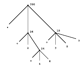
​ Figure 1.1: Tree representation, showing the value of each subcombination.

Next, observe that the repeated application of the first step brings us to the point where we need to evaluate, not combinations, but primitive expressions such as numerals, built-in operators, or other names. We take care of the primitive cases by stipulating that

• the values of numerals are the numbers that they name,
• the values of built-in operators are the machine instruction sequences that carry out the corresponding operations, and
• the values of other names are the objects associated with those names in the environment.

We may regard the second rule as a special case of the third one by stipulating that symbols such as + and * are also included in the global environment, and are associated with the sequences of machine instructions that are their “values.’’ The key point to notice is the role of the environment in determining the meaning of the symbols in expressions. In an interactive language such as Lisp, it is meaningless to speak of the value of an expression such as (+ x 1) without specifying any information about the environment that would provide a meaning for the symbol x (or even for the symbol +). As we shall see in chapter 3, the general notion of the environment as providing a context in which evaluation takes place will play an important role in our understanding of program execution.

Notice that the evaluation rule given above does not handle definitions. For instance, evaluating (define x 3) does not apply define to two arguments, one of which is the value of the symbol x and the other of which is 3, since the purpose of the define is precisely to associate x with a value. (That is, (define x 3) is not a combination.)

Such exceptions to the general evaluation rule are called special forms. Define is the only example of a special form that we have seen so far, but we will meet others shortly. Each special form has its own evaluation rule. The various kinds of expressions (each with its associated evaluation rule) constitute the syntax of the programming language. In comparison with most other programming languages, Lisp has a very simple syntax; that is, the evaluation rule for expressions can be described by a simple general rule together with specialized rules for a small number of special forms.¹¹

1.1.4 Compound Procedures

We have identified in Lisp some of the elements that must appear in any powerful programming language:

• Numbers and arithmetic operations are primitive data and procedures.
• Nesting of combinations provides a means of combining operations.
• Definitions that associate names with values provide a limited means of abstraction.

Now we will learn about procedure definitions, a much more powerful abstraction technique by which a compound operation can be given a name and then referred to as a unit.

We begin by examining how to express the idea of “squaring.” We might say, “To square something, multiply it by itself.’’ This is expressed in our language as

(define (square x) (* x x))

We can understand this in the following way:

(define (square  x)        (*         x     x))

​

To      square something, multiply   it by itself.

We have here a compound procedure, which has been given the name square. The procedure represents the operation of multiplying something by itself. The thing to be multiplied is given a local name, x, which plays the same role that a pronoun plays in natural language. Evaluating the definition creates this compound procedure and associates it with the name square.¹²

The general form of a procedure definition is

(define (<name> <formal parameters>) <body>)

The <*name*> is a symbol to be associated with the procedure definition in the environment.¹³ The <*formal parameters*> are the names used within the body of the procedure to refer to the corresponding arguments of the procedure. The <*body*> is an expression that will yield the value of the procedure application when the formal parameters are replaced by the actual arguments to which the procedure is applied.¹⁴ The <*name*> and the <*formal parameters*> are grouped within parentheses, just as they would be in an actual call to the procedure being defined.

Having defined square, we can now use it:

(square 21)
441

(square (+ 2 5))
49

(square (square 3))
81

We can also use square as a building block in defining other procedures. For example, x2 + y2 can be expressed as

(+ (square x) (square y))

We can easily define a procedure sum-of-squares that, given any two numbers as arguments, produces the sum of their squares:

(define (sum-of-squares x y)
  (+ (square x) (square y)))

(sum-of-squares 3 4)
25

Now we can use sum-of-squares as a building block in constructing further procedures:

(define (f a)
  (sum-of-squares (+ a 1) (* a 2)))

(f 5)
136

Compound procedures are used in exactly the same way as primitive procedures. Indeed, one could not tell by looking at the definition of sum-of-squares given above whether square was built into the interpreter, like + and *, or defined as a compound procedure.

1.1.5 The Substitution Model for Procedure Application

To evaluate a combination whose operator names a compound procedure, the interpreter follows much the same process as for combinations whose operators name primitive procedures, which we described in section ^1.1.3. That is, the interpreter evaluates the elements of the combination and applies the procedure (which is the value of the operator of the combination) to the arguments (which are the values of the operands of the combination).

We can assume that the mechanism for applying primitive procedures to arguments is built into the interpreter. For compound procedures, the application process is as follows:

• To apply a compound procedure to arguments, evaluate the body of the procedure with each formal parameter replaced by the corresponding argument.

To illustrate this process, let’s evaluate the combination

(f 5)

where f is the procedure defined in section 1.1.4. We begin by retrieving the body of f:

(sum-of-squares (+ a 1) (* a 2))

Then we replace the formal parameter a by the argument 5:

(sum-of-squares (+ 5 1) (* 5 2))

Thus the problem reduces to the evaluation of a combination with two operands and an operator sum-of-squares. Evaluating this combination involves three subproblems. We must evaluate the operator to get the procedure to be applied, and we must evaluate the operands to get the arguments. Now (+ 5 1) produces 6 and (* 5 2) produces 10, so we must apply the sum-of-squares procedure to 6 and 10. These values are substituted for the formal parameters x and y in the body of sum-of-squares, reducing the expression to

(+ (square 6) (square 10))

If we use the definition of square, this reduces to

(+ (* 6 6) (* 10 10))

which reduces by multiplication to

(+ 36 100)

and finally to

136

The process we have just described is called the substitution model for procedure application. It can be taken as a model that determines the “meaning’’ of procedure application, insofar as the procedures in this chapter are concerned. However, there are two points that should be stressed:

• The purpose of the substitution is to help us think about procedure application, not to provide a description of how the interpreter really works. Typical interpreters do not evaluate procedure applications by manipulating the text of a procedure to substitute values for the formal parameters. In practice, the “substitution’’ is accomplished by using a local environment for the formal parameters. We will discuss this more fully in chapters 3 and 4 when we examine the implementation of an interpreter in detail.
• Over the course of this book, we will present a sequence of increasingly elaborate models of how interpreters work, culminating with a complete implementation of an interpreter and compiler in chapter 5. The substitution model is only the first of these models – a way to get started thinking formally about the evaluation process. In general, when modeling phenomena in science and engineering, we begin with simplified, incomplete models. As we examine things in greater detail, these simple models become inadequate and must be replaced by more refined models. The substitution model is no exception. In particular, when we address in chapter 3 the use of procedures with ``mutable data,’’ we will see that the substitution model breaks down and must be replaced by a more complicated model of procedure application.¹⁵

Applicative order versus normal order

According to the description of evaluation given in section ^1.1.3, the interpreter first evaluates the operator and operands and then applies the resulting procedure to the resulting arguments. This is not the only way to perform evaluation. An alternative evaluation model would not evaluate the operands until their values were needed. Instead it would first substitute operand expressions for parameters until it obtained an expression involving only primitive operators, and would then perform the evaluation. If we used this method, the evaluation of

(f 5)

would proceed according to the sequence of expansions

(sum-of-squares (+ 5 1) (* 5 2))

(+    (square (+ 5 1))      (square (* 5 2))  )

(+    (* (+ 5 1) (+ 5 1))   (* (* 5 2) (* 5 2)))

followed by the reductions

(+         (* 6 6)             (* 10 10))

(+           36                   100)

                    136

This gives the same answer as our previous evaluation model, but the process is different. In particular, the evaluations of (+ 5 1) and (* 5 2) are each performed twice here, corresponding to the reduction of the expression

(* x x)

with x replaced respectively by (+ 5 1) and (* 5 2).

This alternative “fully expand and then reduce’’ evaluation method is known as normal-order evaluation, in contrast to the “evaluate the arguments and then apply’’ method that the interpreter actually uses, which is called applicative-order evaluation. It can be shown that, for procedure applications that can be modeled using substitution (including all the procedures in the first two chapters of this book) and that yield legitimate values, normal-order and applicative-order evaluation produce the same value. (See exercise ^1.5 for an instance of an “illegitimate’’ value where normal-order and applicative-order evaluation do not give the same result.)

Lisp uses applicative-order evaluation, partly because of the additional efficiency obtained from avoiding multiple evaluations of expressions such as those illustrated with (+ 5 1) and (* 5 2) above and, more significantly, because normal-order evaluation becomes much more complicated to deal with when we leave the realm of procedures that can be modeled by substitution. On the other hand, normal-order evaluation can be an extremely valuable tool, and we will investigate some of its implications in chapters 3 and 4.¹⁶

1.1.6 Conditional Expressions and Predicates

The expressive power of the class of procedures that we can define at this point is very limited, because we have no way to make tests and to perform different operations depending on the result of a test. For instance, we cannot define a procedure that computes the absolute value of a number by testing whether the number is positive, negative, or zero and taking different actions in the different cases according to the rule

This construct is called a case analysis, and there is a special form in Lisp for notating such a case analysis. It is called cond (which stands for “conditional’’), and it is used as follows:

(define (abs x)
  (cond ((> x 0) x)
        ((= x 0) 0)
        ((< x 0) (- x))))

The general form of a conditional expression is

(cond (<p1> <e1>)
      (<p2> <e2>)
      
      (<pn> <en>))

consisting of the symbol cond followed by parenthesized pairs of expressions (<p> <e>) called clauses. The first expression in each pair is a predicate – that is, an expression whose value is interpreted as either true or false.¹⁷

Conditional expressions are evaluated as follows. The predicate <*p1*> is evaluated first. If its value is false, then <*p2*> is evaluated. If <*p2*>’s value is also false, then <*p3*> is evaluated. This process continues until a predicate is found whose value is true, in which case the interpreter returns the value of the corresponding consequent expression <*e*> of the clause as the value of the conditional expression. If none of the <*p*>’s is found to be true, the value of the cond is undefined.

The word predicate is used for procedures that return true or false, as well as for expressions that evaluate to true or false. The absolute-value procedure abs makes use of the primitive predicates >, <, and =.¹⁸ These take two numbers as arguments and test whether the first number is, respectively, greater than, less than, or equal to the second number, returning true or false accordingly.

Another way to write the absolute-value procedure is

(define (abs x)
  (cond ((< x 0) (- x))
        (else x)))

which could be expressed in English as “If x is less than zero return - x; otherwise return x.’’ Else is a special symbol that can be used in place of the <*p*> in the final clause of a cond. This causes the cond to return as its value the value of the corresponding <*e*> whenever all previous clauses have been bypassed. In fact, any expression that always evaluates to a true value could be used as the <*p*> here.

Here is yet another way to write the absolute-value procedure:

(define (abs x)
  (if (< x 0)
      (- x)
      x))

This uses the special form if, a restricted type of conditional that can be used when there are precisely two cases in the case analysis. The general form of an if expression is

(if <predicate> <consequent> <alternative>)

To evaluate an if expression, the interpreter starts by evaluating the <*predicate*> part of the expression. If the <*predicate*> evaluates to a true value, the interpreter then evaluates the <*consequent*> and returns its value. Otherwise it evaluates the <*alternative*> and returns its value.¹⁹

In addition to primitive predicates such as <, =, and >, there are logical composition operations, which enable us to construct compound predicates. The three most frequently used are these:

• (and <*e1*> ... <*en*>)

  The interpreter evaluates the expressions <*e*> one at a time, in left-to-right order. If any <*e*> evaluates to false, the value of the and expression is false, and the rest of the <*e*>’s are not evaluated. If all <*e*>’s evaluate to true values, the value of the and expression is the value of the last one.

• (or <*e1*> ... <*en*>)

  The interpreter evaluates the expressions <*e*> one at a time, in left-to-right order. If any <*e*> evaluates to a true value, that value is returned as the value of the or expression, and the rest of the <*e*>’s are not evaluated. If all <*e*>’s evaluate to false, the value of the or expression is false.

• (not <*e*>)

  The value of a not expression is true when the expression <*e*> evaluates to false, and false otherwise.

Notice that and and or are special forms, not procedures, because the subexpressions are not necessarily all evaluated. Not is an ordinary procedure.

As an example of how these are used, the condition that a number x be in the range 5 < x < 10 may be expressed as

(and (> x 5) (< x 10))

As another example, we can define a predicate to test whether one number is greater than or equal to another as

(define (>= x y)
  (or (> x y) (= x y)))

or alternatively as

(define (>= x y)
  (not (< x y)))

Exercise 1.1. Below is a sequence of expressions. What is the result printed by the interpreter in response to each expression? Assume that the sequence is to be evaluated in the order in which it is presented.

10
(+ 5 3 4)
(- 9 1)
(/ 6 2)
(+ (* 2 4) (- 4 6))
(define a 3)
(define b (+ a 1))
(+ a b (* a b))
(= a b)
(if (and (> b a) (< b (* a b)))
    b
    a)
(cond ((= a 4) 6)
      ((= b 4) (+ 6 7 a))
      (else 25))
(+ 2 (if (> b a) b a))
(* (cond ((> a b) a)
         ((< a b) b)
         (else -1))
   (+ a 1))

answer:

10
12
8
3
6
19
#f
4
16
6
16

Exercise 1.2. Translate the following expression into prefix form

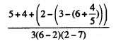
answer:

#lang sicp

(/ (+ 5 4
      (- 2
         (- 3
            (+ 6
               (/ 4 5)
               )
            )
         )
      )
   (* 3
      (- 6 2)
      (- 2 7)
      )
   )

-37/150

Exercise 1.3. Define a procedure that takes three numbers as arguments and returns the sum of the squares of the two larger numbers.

answer:

#lang sicp

(define (square x) (* x x))
(define (sum-of-squares x y) (+ (square x) (square y)))
(define (fn x y z)
  (cond ((and (< x y) (< x z)) (sum-of-squares y z))
        ((and (< y x) (< y z)) (sum-of-squares x z))
        ((and (< z x) (< z y)) (sum-of-squares x y))
        ))
(fn 3 2 1)

Exercise 1.4. Observe that our model of evaluation allows for combinations whose operators are compound expressions. Use this observation to describe the behavior of the following procedure:

(define (a-plus-abs-b a b)
  ((if (> b 0) + -) a b))

Exercise 1.5. Ben Bitdiddle has invented a test to determine whether the interpreter he is faced with is using applicative-order evaluation or normal-order evaluation. He defines the following two procedures:

(define (p) (p))

(define (test x y)
  (if (= x 0)
      0
      y))

Then he evaluates the expression

(test 0 (p))

What behavior will Ben observe with an interpreter that uses applicative-order evaluation? What behavior will he observe with an interpreter that uses normal-order evaluation? Explain your answer. (Assume that the evaluation rule for the special form if is the same whether the interpreter is using normal or applicative order: The predicate expression is evaluated first, and the result determines whether to evaluate the consequent or the alternative expression.)

1.1.7 Example: Square Roots by Newton’s Method

Procedures, as introduced above, are much like ordinary mathematical functions. They specify a value that is determined by one or more parameters. But there is an important difference between mathematical functions and computer procedures. Procedures must be effective.

As a case in point, consider the problem of computing square roots. We can define the square-root function as

This describes a perfectly legitimate mathematical function. We could use it to recognize whether one number is the square root of another, or to derive facts about square roots in general. On the other hand, the definition does not describe a procedure. Indeed, it tells us almost nothing about how to actually find the square root of a given number. It will not help matters to rephrase this definition in pseudo-Lisp:

(define (sqrt x)
  (the y (and (>= y 0)
              (= (square y) x))))

This only begs the question.

The contrast between function and procedure is a reflection of the general distinction between describing properties of things and describing how to do things, or, as it is sometimes referred to, the distinction between declarative knowledge and imperative knowledge. In mathematics we are usually concerned with declarative (what is) descriptions, whereas in computer science we are usually concerned with imperative (how to) descriptions.²⁰

How does one compute square roots? The most common way is to use Newton’s method of successive approximations, which says that whenever we have a guess y for the value of the square root of a number x, we can perform a simple manipulation to get a better guess (one closer to the actual square root) by averaging y with x/y.²¹ For example, we can compute the square root of 2 as follows. Suppose our initial guess is 1:

Guess	Quotient	Average
1	(2/1) = 2	((2 + 1)/2) = 1.5
1.5	(2/1.5) = 1.3333	((1.3333 + 1.5)/2) = 1.4167
1.4167	(2/1.4167) = 1.4118	((1.4167 + 1.4118)/2) = 1.4142
1.4142	...	...

Continuing this process, we obtain better and better approximations to the square root.

Now let’s formalize the process in terms of procedures. We start with a value for the radicand (the number whose square root we are trying to compute) and a value for the guess. If the guess is good enough for our purposes, we are done; if not, we must repeat the process with an improved guess. We write this basic strategy as a procedure:

(define (sqrt-iter guess x)
  (if (good-enough? guess x)
      guess
      (sqrt-iter (improve guess x)
                 x)))

A guess is improved by averaging it with the quotient of the radicand and the old guess:

(define (improve guess x)
  (average guess (/ x guess)))

where

(define (average x y)
  (/ (+ x y) 2))

We also have to say what we mean by “good enough.’’ The following will do for illustration, but it is not really a very good test. (See exercise ^1.7.) The idea is to improve the answer until it is close enough so that its square differs from the radicand by less than a predetermined tolerance (here 0.001):²²

(define (good-enough? guess x)
  (< (abs (- (square guess) x)) 0.001))

Finally, we need a way to get started. For instance, we can always guess that the square root of any number is 1:²³

(define (sqrt x)
  (sqrt-iter 1.0 x))

If we type these definitions to the interpreter, we can use sqrt just as we can use any procedure:

(sqrt 9)
3.00009155413138
(sqrt (+ 100 37))
11.704699917758145
(sqrt (+ (sqrt 2) (sqrt 3)))
1.7739279023207892
(square (sqrt 1000))
1000.000369924366

The sqrt program also illustrates that the simple procedural language we have introduced so far is sufficient for writing any purely numerical program that one could write in, say, C or Pascal. This might seem surprising, since we have not included in our language any iterative (looping) constructs that direct the computer to do something over and over again. Sqrt-iter, on the other hand, demonstrates how iteration can be accomplished using no special construct other than the ordinary ability to call a procedure.²⁴

完整代码：

#lang sicp

(define (>= x y)
  (or (> x y) (= x y)))

(define (average x y)
  (/ (+ x y) 2))

(define (improve guess x)
  (average guess (/ x guess)))

(define (square x) (* x x))

(define (abs x)
  (cond ((> x 0) x)
        ((= x 0) 0)
        ((< x 0) (- x))))

(define (good-enough? guess x)
  (< (abs (- (square guess) x)) 0.001))



(define (sqrt-iter guess x)
  (if (good-enough? guess x)
      guess
      (sqrt-iter (improve guess x)
                 x)))

(define (sqrt x)
  (sqrt-iter 1.0 x))

(sqrt 9)
(sqrt (+ 100 37))
(sqrt (+ (sqrt 2) (sqrt 3)))
(square (sqrt 1000))

Exercise 1.6. Alyssa P. Hacker doesn’t see why if needs to be provided as a special form. Why can't I just define it as an ordinary procedure in terms of "cond" ? she asks. Alyssa’s friend Eva Lu Ator claims this can indeed be done, and she defines a new version of if:

(define (new-if predicate then-clause else-clause)
  (cond (predicate then-clause)
        (else else-clause)))

Eva demonstrates the program for Alyssa:

(new-if (= 2 3) 0 5)
5

(new-if (= 1 1) 0 5)
0

Delighted, Alyssa uses new-if to rewrite the square-root program:

(define (sqrt-iter guess x)
  (new-if (good-enough? guess x)
          guess
          (sqrt-iter (improve guess x)
                     x)))

What happens when Alyssa attempts to use this to compute square roots? Explain.

Exercise 1.7. The good-enough? test used in computing square roots will not be very effective for finding the square roots of very small numbers. Also, in real computers, arithmetic operations are almost always performed with limited precision. This makes our test inadequate for very large numbers. Explain these statements, with examples showing how the test fails for small and large numbers. An alternative strategy for implementing good-enough? is to watch how guess changes from one iteration to the next and to stop when the change is a very small fraction of the guess. Design a square-root procedure that uses this kind of end test. Does this work better for small and large numbers?

Exercise 1.8. Newton’s method for cube roots is based on the fact that if y is an approximation to the cube root of x, then a better approximation is given by the valueUse this formula to implement a cube-root procedure analogous to the square-root procedure. (In section ^1.3.4 we will see how to implement Newton’s method in general as an abstraction of these square-root and cube-root procedures.)